An R6 class implementing slicing window for offline change-point detection.
Details
Slicing window is a scalable, linear-time change-point detection algorithm that selects breakpoints based on local gains computed over sliding windows.
Currently supports the following cost functions:
"L1"and"L2"for (independent) piecewise Gaussian process with constant variance"SIGMA": for (independent) piecewise Gaussian process with varying variance"VAR": for piecewise Gaussian vector-regressive process with constant noise variance"LinearL2": for piecewise linear regression process with constant noise variance"LinearSIGMA": for piecewise linear regression process with varying noise covariance"LinearL1": for piecewise linear regression process under L1 (least absolute deviations) loss
Window requires a R6 object of class costFunc, which can be created via costFunc$new(). Currently, the following cost functions are supported:
"L1"and"L2"for (independent) piecewise Gaussian process with constant variance"SIGMA": for (independent) piecewise Gaussian process with varying variance"VAR": for piecewise Gaussian vector-regressive process with constant noise variance"LinearL2": for piecewise linear regression process with constant noise variance"LinearSIGMA": for piecewise linear regression process with varying noise covariance"LinearL1": for piecewise linear regression process under L1 (least absolute deviations) loss
See $eval() method for more details on computation of cost.
Some examples are provided below. See the package website for detailed usage!
Methods
$new()Initialises a
Windowobject.$describe()Describes the
Windowobject.$fit()Constructs a
Windowmodule inC++.$eval()Evaluates the cost of a segment.
$predict()Performs
Windowgiven a linear penalty value.$segments()Returns the cost and parameter estimates of each segment from the latest
$predict().$getHistory()Retrieves the full cost history and sequentially added breakpoints.
$plotElbow()Plots the elbow curve (Total Cost vs. Number of Change-Points).
$plot()Plots change-point segmentation in
ggplotstyle.$clone()Clones the
R6object.
References
Truong, C., Oudre, L., & Vayatis, N. (2020). Selective review of offline change point detection methods. Signal Processing, 167, 107299.
Author
Minh Long Nguyen edelweiss611428@gmail.com
Toby Dylan Hocking toby.hocking@r-project.org
Charles Truong ctruong@ens-paris-saclay.fr
Huy Nhat Minh Nguyen sleepysnorlax0115@gmail.com
Active bindings
minSizeInteger. Minimum allowed segment length. Can be accessed or modified via
$minSize. ModifyingminSizewill automatically trigger$fit().radiusInteger. Window radius. Can be accessed or modified via
$radius. Modifyingradiuswill automatically trigger$fit().jumpInteger. Search grid step size. Can be accessed or modified via
$jump. Modifyingjumpwill automatically trigger$fit().costFuncR6object of classcostFunc. Search grid step size. Can be accessed or modified via$costFunc. ModifyingcostFuncwill automatically trigger$fit().tsMatNumeric matrix. Input time series matrix of size \(n \times p\). Can be accessed or modified via
$tsMat. ModifyingtsMatwill automatically trigger$fit().covariatesNumeric matrix. Input time series matrix having a similar number of observations as
tsMat. Can be accessed or modified via$covariates. Modifyingcovariateswill automatically trigger$fit().
Methods
Method new()
Initialises a Window object.
Usage
Window$new(minSize, jump, radius, costFunc)Arguments
minSizeInteger. Minimum allowed segment length. Default:
1L.jumpInteger. Search grid step size: only positions in {k, 2k, ...} are considered. Default:
1L.radiusInteger. Radius of each sliding window. Default:
1L.costFuncA
R6object of classcostFunc. Should be created viacostFunc$new()to avoid error. Default:costFunc$new("L2").
Method describe()
Describes a Window object.
Returns
Invisibly returns a list storing at least the following fields:
minSizeMinimum allowed segment length.
jumpSearch grid step size.
radiusRadius of each sliding window.
costFuncThe
costFuncobject.fittedWhether or not
$fit()has been run.tsMatTime series matrix.
covariatesCovariate matrix (if exists).
nNumber of observations.
pNumber of features.
Method fit()
Constructs a C++ module for Window.
Arguments
tsMatNumeric matrix. A time series matrix of size \(n \times p\) whose rows are observations ordered in time. If
tsMat = NULL, the method will use the previously assignedtsMat(e.g., set via the active binding$tsMator from a prior$fit(tsMat)). Default:NULL.covariatesNumeric matrix. A time series matrix having a similar number of observations as
tsMat. Required for models involving both dependent and independent variables. Ifcovariates = NULLand no prior covariates were set (i.e.,$covariatesis stillNULL), the model is force-fitted with only an intercept. Default:NULL..
Method eval()
Evaluate the cost of the segment (a,b]
Arguments
aInteger. Start index of the segment (exclusive). Must satisfy
start < end.bInteger. End index of the segment (inclusive).
Details
The segment cost is evaluated as follows:
L1 cost function: $$c_{L_1}(y_{(a+1)...b}) := \sum_{t = a+1}^{b} \| y_t - \tilde{y}_{(a+1)...b} \|_1$$ where \(\tilde{y}_{(a+1)...b}\) is the coordinate-wise median of the segment. If \(a \ge b - 1\), return 0.
L2 cost function: $$c_{L_2}(y_{(a+1)...b}) := \sum_{t = a+1}^{b} \| y_t - \bar{y}_{(a+1)...b} \|_2^2$$ where \(\bar{y}_{(a+1)...b}\) is the empirical mean of the segment. If \(a \ge b - 1\), return 0.
SIGMA cost function: $$c_{\Sigma}(y_{(a+1)...b}) := (b - a)\log \det \hat{\Sigma}_{(a+1)...b}$$ where \(\hat{\Sigma}_{(a+1)...b}\) is the empirical covariance matrix of the segment without Bessel's correction. Here, if
addSmallDiag = TRUE, a small biasepsilonis added to the diagonal of estimated covariance matrices to improve numerical stability.
By default,addSmallDiag = TRUEandepsilon = 1e-6. In caseaddSmallDiag = TRUE, if the covariance matrix is numerically singular (its log-determinant cannot be computed) or its log-determinant is smaller than the lower boundp*log(epsilon), return(b - a)*p*log(epsilon), otherwise, output an error message.VAR(r) cost function: $$c_{\mathrm{VAR}}(y_{(a+1)...b}) := \sum_{t = \max(a, r)+1}^{b} \left\| y_t - \hat c - \sum_{j=1}^r \hat A_j y_{t-j} \right\|_2^2$$ where \(\hat c\) and \(\hat A_j\) are the OLS estimates of the intercept and VAR coefficients on the segment. The lagged values \(y_{t-j}\) may come from before \(a+1\), so only the first \(r\) observations of the whole series lack a full set of lags. If the system is singular, an approximate (minimum-norm) least-squares solve is used. If \(b-a < p*r+1\) (i.e., not enough observations), or \(a > n-r\) (where
nis the time series length), return 0."LinearL2" for piecewise linear regression process with constant noise variance $$c_{\text{LinearL2}}(y_{(a+1):b}) := \sum_{t=a+1}^b \| y_t - X_t \hat{\beta} \|_2^2$$ where \(\hat{\beta}\) are OLS estimates on segment \((a+1):b\). If segment is shorter than the minimum number of points needed for OLS, return 0.
"LinearSIGMA" for piecewise linear regression process with varying noise covariance $$c_{\text{LinearSIGMA}}(y_{(a+1):b}) := (b-a)\log \det \hat\Sigma_{(a+1):b}$$ where \(\hat\Sigma_{(a+1):b}\) is the empirical covariance matrix of OLS residuals \(y - X\hat{\beta}\) on segment \((a+1):b\), divided by \(b-a\) with no degrees-of-freedom correction for the fitted coefficients, and otherwise estimated the same way as in the SIGMA cost function.
"LinearL1" for piecewise linear regression process under L1 (least absolute deviations) loss $$c_{\text{LinearL1}}(y_{(a+1):b}) := \sum_{t=a+1}^b \| y_t - X_t \hat{\beta} \|_1$$ where \(\hat{\beta}\) is fit column-by-column via IRLS on segment \((a+1):b\), iterated until convergence (
tol) ormaxIter. Unlike the other regression costs, this has no \(O(1)\)-per-segment closed form.
Method predict()
Performs Window given a linear penalty value, or a target number of change-points.
Arguments
penNumeric. Penalty per change-point. Ignored if
nBkpsis supplied. Default:0.nBkpsInteger. If supplied, takes precedence over
pen: returns thenBkpshighest-gain local maxima found by$fit()(see$getHistory()), i.e.Window's own best answer for that many change-points – not necessarily the globally optimal one for that count (seeDynpfor that guarantee). Treated as an upper bound, not a strict requirement:Windowonly ever finds finitely many local maxima, so if fewer thannBkpsexist, all of them are returned and a message reports the shortfall. Default:NULL.
Details
The algorithm scans the data with a fixed-size window to detect candidate local change-points (lcps) if the gains of its \(k_\text{thresh}\) neighbors to the left and right are all smaller than its gain, where \(k_\text{thresh}\) is defined as $$ k_\text{thresh} = \max \left( \left\lfloor \frac{\max(2\text{radius}, 2 \cdot \text{minSize})}{2 \cdot \text{jump}} \right\rfloor, 1 \right) $$
After candidate local change-points and computing the local gains, the algorithm selects the "optimal" set of break-points given the linear penalty threshold. Let \(G_i\) denote the local gain for candidate change-point \(i\), for \(i = 1, \dots, n_\text{lcps}\). The local gains are ordered such that \(G_1 \ge G_2 \ge \dots \ge G_{n_\text{lcps}}\). Note that it is possible that no local change-points are detected, for example if the window size is too large.
The total cost for the selected \(k\) change-points is then calculated as $$ \text{TotalCost} = - \sum_{i=1}^{k} G_i + \lambda \cdot k, $$ where \(\lambda\) is a linear penalty applied per change-point. We then optimise over \(k = 1, \dots, n_\text{lcps}\) to minimise the penalised cost function. \(k = 0\) is not a candidate, so at least one change-point is returned whenever a local change-point exists, however large the penalty.
This approach allows detecting multiple change-points in a time series while controlling model complexity through the linear penalty threshold.
In our implementation, scanning the data to detect candidate local change-points and computing their corresponding local gains is already performed in $fit().
Therefore, $predict() runs in linear time with respect to the number of local change-points.
Temporary segment end-points are saved to private$.tmpEndPoints after $predict(), enabling users to call $plot() without
specifying endpoints manually.
Method segments()
Returns the cost and parameter estimates of each segment from the latest $predict().
Details
Let \(0 = c_0 < c_1 < \dots < c_{k+1} = n\) be the end-points from the latest $predict(), called with either
pen or nBkps. Segment \(i\) is \((c_{i-1}, c_i]\), Cost is \(c_{(c_{i-1}, c_i]}\) and Params is its
minimiser. The costs sum to the total cost of this segmentation. For \(k \ge 1\) this generally differs from
$getHistory()$cost[k + 1], which subtracts local gains computed on windows of 2 * radius points instead of
re-evaluating the segments.
Temporary end-points are cleared by $fit(), so $predict() must be run again after modifying the object via
its active bindings.
Returns
A list with one element per segment \((Start, End]\). Each element is a list with:
StartStart index of the segment (exclusive, 0-based), same convention as
$eval().EndEnd index of the segment (inclusive).
CostThe segment cost, as returned by
$eval(Start, End).ParamsA named list of the segment parameter estimates, e.g.
list(mean = ...)for"L2". SeecostFactoryfor the fields returned by each cost function.
Method plotElbow()
Plots the elbow curve (Total Cost vs. Number of Change-Points).
Method plot()
Plots change-point segmentation
Usage
Window$plot(
  d = 1L,
  endPts,
  dimNames,
  main,
  xlab,
  tsWidth = 0.25,
  tsCol = "#5B9BD5",
  bgCol = c("#A3C4F3", "#FBB1BD"),
  bgAlpha = 0.5,
  ncol = 1L
)
Arguments
dInteger vector. Dimensions to plot. Default:
1L.endPtsInteger vector. End points. Default: latest temporary changepoints obtained via
$predict().dimNamesCharacter vector. Feature names matching length of
d. Defaults to"X1", "X2", ....mainCharacter. Main title. Defaults to
"Window: d = ...".xlabCharacter. X-axis label. Default:
"Time".tsWidthNumeric. Line width for time series and segments. Default:
0.25.tsColCharacter. Time series color. Default:
"#5B9BD5".bgColCharacter vector. Segment colors, recycled to length of
endPts. Default:c("#A3C4F3", "#FBB1BD").bgAlphaNumeric. Background transparency. Default:
0.5.ncolInteger. Number of columns in facet layout. Default:
1L.
Examples
## L2 example
set.seed(1121)
signals = as.matrix(c(rnorm(100,0,1),
rnorm(100,5,1)))
# Default L2 cost function
WindowObj = Window$new(minSize = 1L, jump = 1L)
WindowObj$fit(signals)
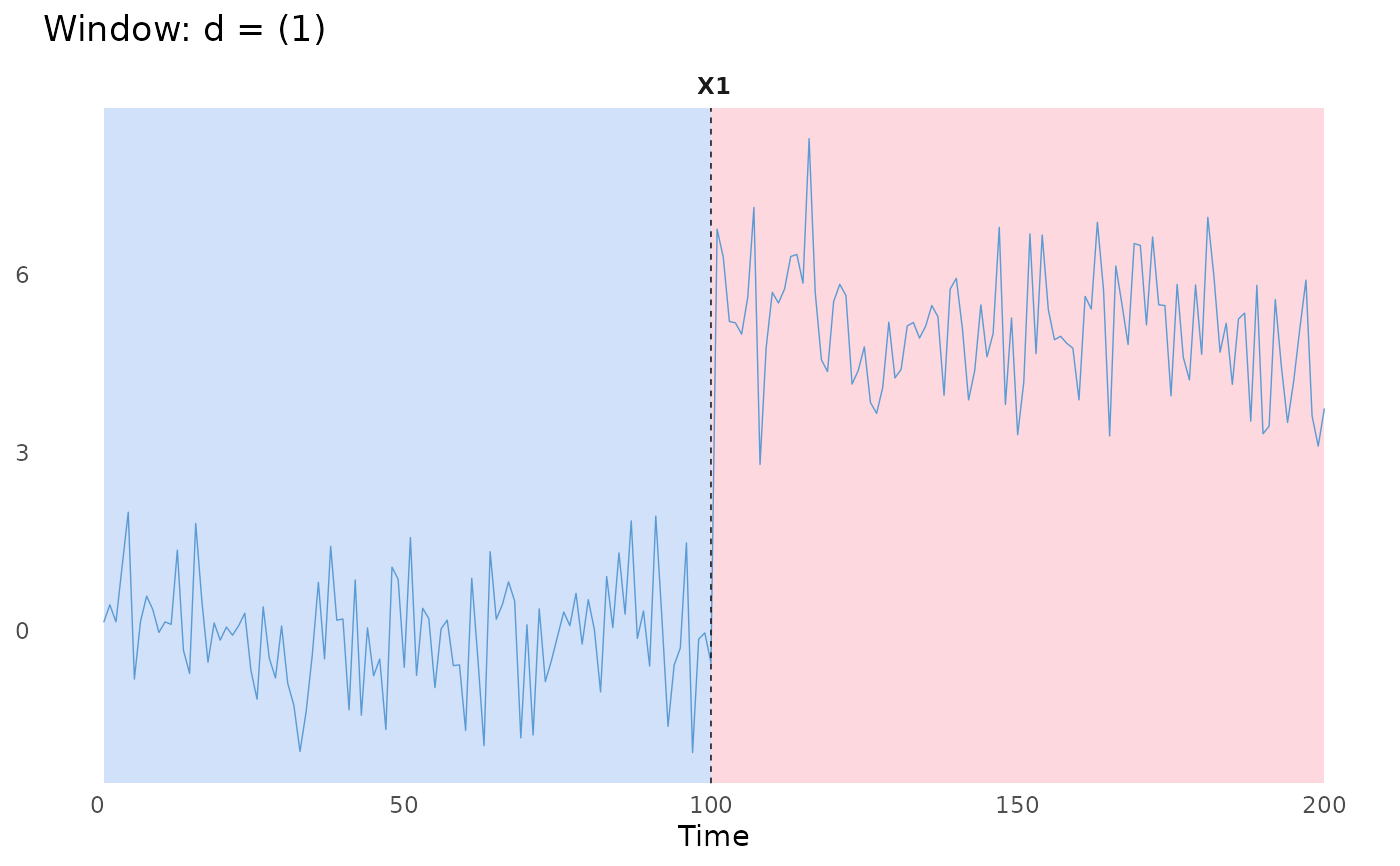
WindowObj$predict(pen = 100)
#> [1] 100 200
WindowObj$plot()
#> `endPts` is missing. Proceed to use the temporary `endPts`!
#> `dimNames` is missing. Proceed to use the default `dimNames`! e.g., `paste0('X', d))`.
 ## SIGMA example
set.seed(111)
signals = as.matrix(c(rnorm(100,-5,1),
rnorm(100,-5,10),
rnorm(100,-5,1)))
# L2 cost function
WindowObj = Window$new(minSize = 1L, jump = 1L)
WindowObj$fit(signals)
# We choose pen = 50.
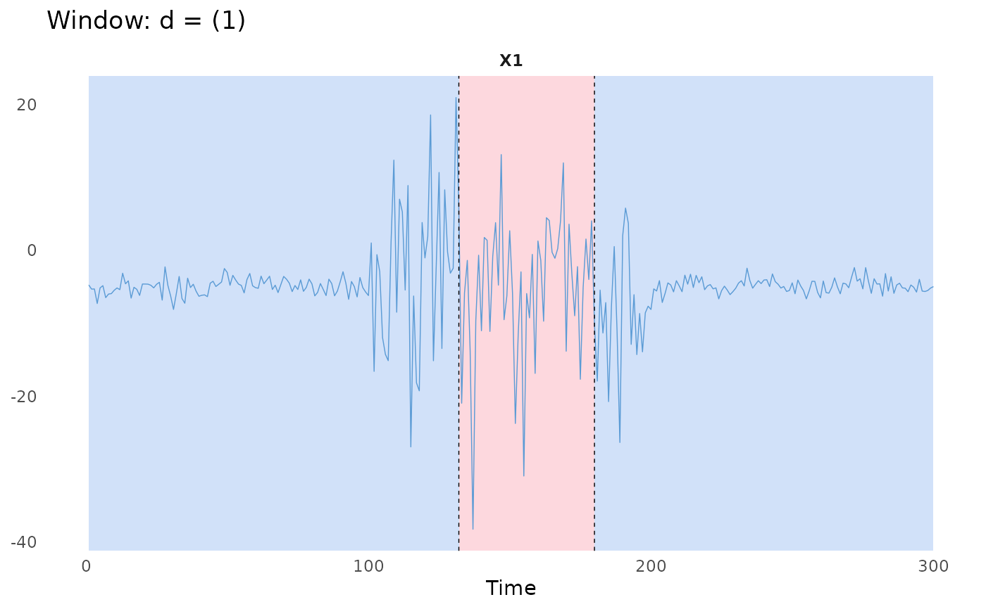
WindowObj$predict(pen = 50)
#> [1] 132 180 300
WindowObj$plot()
#> `endPts` is missing. Proceed to use the temporary `endPts`!
#> `dimNames` is missing. Proceed to use the default `dimNames`! e.g., `paste0('X', d))`.
## SIGMA example
set.seed(111)
signals = as.matrix(c(rnorm(100,-5,1),
rnorm(100,-5,10),
rnorm(100,-5,1)))
# L2 cost function
WindowObj = Window$new(minSize = 1L, jump = 1L)
WindowObj$fit(signals)
# We choose pen = 50.
WindowObj$predict(pen = 50)
#> [1] 132 180 300
WindowObj$plot()
#> `endPts` is missing. Proceed to use the temporary `endPts`!
#> `dimNames` is missing. Proceed to use the default `dimNames`! e.g., `paste0('X', d))`.
 # The standard L2 cost function is not suitable.
# Use the SIGMA cost function.
WindowObj$costFunc = costFunc$new(costFunc = "SIGMA")
#> `costFunc` has been updated. Re-fitting the model.
WindowObj$predict(pen = 50)
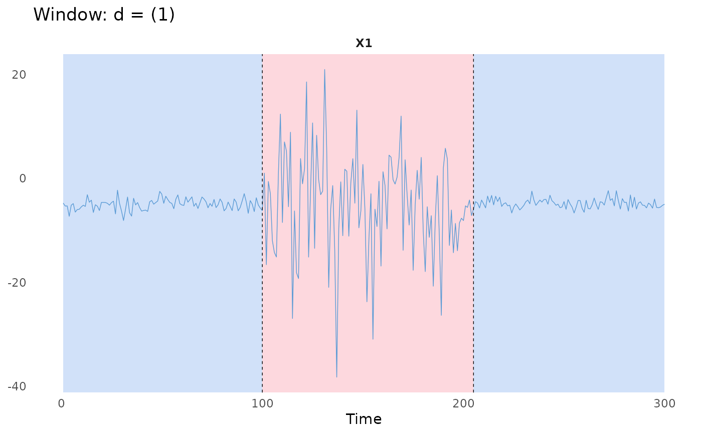
#> [1] 100 205 300
WindowObj$plot()
#> `endPts` is missing. Proceed to use the temporary `endPts`!
#> `dimNames` is missing. Proceed to use the default `dimNames`! e.g., `paste0('X', d))`.
# The standard L2 cost function is not suitable.
# Use the SIGMA cost function.
WindowObj$costFunc = costFunc$new(costFunc = "SIGMA")
#> `costFunc` has been updated. Re-fitting the model.
WindowObj$predict(pen = 50)
#> [1] 100 205 300
WindowObj$plot()
#> `endPts` is missing. Proceed to use the temporary `endPts`!
#> `dimNames` is missing. Proceed to use the default `dimNames`! e.g., `paste0('X', d))`.