Change in mean and variance

This case study detects a change in mean and variance in a simulated two-dimensional series, with the "SIGMA" cost and binary segmentation (binSeg).

library(rupturesRcpp)

To demonstrate the package usage, we first consider a simple 2d time series with two piecewise Gaussian regimes and varying variance.

set.seed(1)
tsMat = cbind(c(rnorm(100,0), rnorm(100,5,5)),
              c(rnorm(100,0), rnorm(100,5,5)))

As our example involves regimes with varying variance, a suitable costFunc option is "SIGMA". Since the segmentation objects’ interfaces are similar, it is sufficient to demonstrate the usage of binSeg only.

SIGMAObj = costFunc$new("SIGMA", addSmallDiag = TRUE, epsilon = 1e-6)
binSegObj = binSeg$new(minSize = 1L, jump = 1L, costFunc = SIGMAObj)
binSegObj$fit(tsMat)

Once fitted, $predict() and $eval() can be used. To view the configurations of the binSeg object, we can use $describe().

binSegObj$describe(printConfig = TRUE)
#> Binary Segmentation (binSeg) 
#> minSize      : 1L
#> jump         : 1L
#> costFunc     : "SIGMA"
#> addSmallDiag : TRUE
#> epsilon      : 1e-06
#> fitted       : TRUE
#> n            : 200L
#> p            : 2L

To obtain an estimated segmentation, we can use the $predict() method and specify a non-negative penalty value pen, which should be properly tuned. This returns a sorted integer vector of end-points, including the number of observations by design.

Here, we set pen = 100 by hand. See Tuning the penalty for how pen could be tuned.

binSegObj$predict(pen = 100)
#> [1] 100 200

After running $predict(), the segmentation output is temporarily saved to the binSeg object, allowing users to use the $plot() method without specifying endPts.

binSegObj$plot(d = 1:2,
               main = "method: binSeg; costFunc: SIGMA; pen: 100")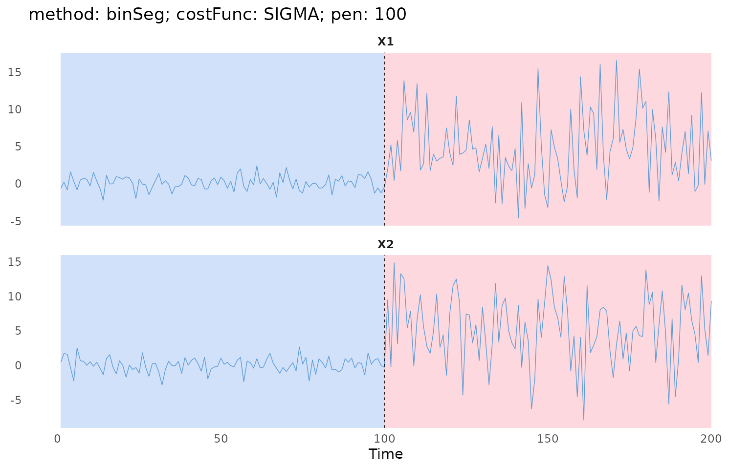

Instead of setting pen, we can choose the number of change-points with the elbow method (see Model selection). $plotElbow() plots the cost against the number of change-points.

binSegObj$plotElbow(maxK = 10)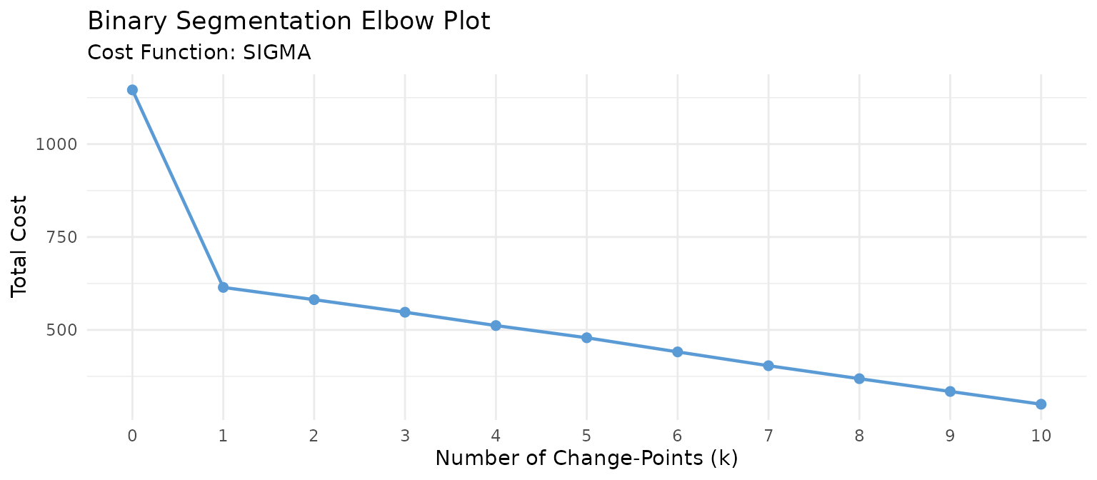

The cost drops sharply at one change-point and then falls only slowly, so we take nBkps = 1. This gives the same change-point as pen = 100.

binSegObj$predict(nBkps = 1)
#> [1] 100 200