Custom cost functions

This case study writes cost functions in R with costFunc$new("Custom", ...) (see User-defined cost functions). It checks one against a built-in cost, uses data that were never passed to $fit(), and shows the risk that comes with that.

library(rupturesRcpp)

Checking against a built-in cost

As a sanity check, re-implementing "L2" as a "Custom" cost gives identical numbers:

myL2eval = function(segment, a, b){
  segment = as.matrix(segment)
  cm = colMeans(segment)
  sum(sweep(segment, 2, cm, FUN = "-")^2)
}

customCF = costFunc$new("Custom", evalFun = myL2eval)
customCF$pass()
#> $costFunc
#> [1] "Custom"
#> 
#> $evalFun
#> function (segment, a, b) 
#> {
#>     segment = as.matrix(segment)
#>     cm = colMeans(segment)
#>     sum(sweep(segment, 2, cm, FUN = "-")^2)
#> }
#> 
#> $paramFun
#> NULL

set.seed(1)
tsMat = cbind(c(rnorm(100,0), rnorm(100,5,5)),
              c(rnorm(100,0), rnorm(100,5,5))) # the series from the mean and variance case study

customObj = PELT$new(minSize = 1L, jump = 1L, costFunc = customCF)
customObj$fit(tsMat)
customObj$eval(0, 150)
#> [1] 3943.78

which matches

L2Obj = PELT$new(costFunc = costFunc$new("L2"))
L2Obj$fit(tsMat)
L2Obj$eval(0, 150)
#> [1] 3943.78

exactly.

Using external data

The actual use case is a custom cost function that closes over data the package was never explicitly given. For example, below, externalSeries is captured purely through lexical scope (it is never passed to $fit()), and evalFun uses a and b to align it with each candidate segment:

set.seed(1)
tsMat2 = cbind(c(rnorm(100, 0), rnorm(100, 4)))
externalSeries = as.matrix(rnorm(200)) # captured by closure, never passed to `$fit()`

externalRegCost = function(segment, a, b){
  x = externalSeries[(a+1):b, , drop = FALSE]
  sum(lm(segment ~ x)$residuals^2)
}

customObj2 = PELT$new(minSize = 2L, jump = 1L,
                       costFunc = costFunc$new("Custom", evalFun = externalRegCost))
customObj2$fit(tsMat2)
customObj2$predict(pen = 15)
#> [1] 100 200

This matches the built-in "LinearL2" cost told about externalSeries directly, via covariates:

linObj = PELT$new(minSize = 2L, jump = 1L, costFunc = costFunc$new("LinearL2"))
linObj$fit(tsMat2, externalSeries)
linObj$predict(pen = 15)
#> [1] 100 200

$describe() reports evalFun/paramFun as <function>/NULL rather than printing the closure itself:

customObj2$describe(printConfig = TRUE)
#> Pruned Exact Linear Time (PELT) 
#> minSize      : 2L
#> jump         : 1L
#> costFunc     : "Custom"
#> evalFun      : <function>
#> paramFun     : NULL
#> fitted       : TRUE
#> n            : 200L
#> p            : 1L

Risk of data mismatch

The segmentation logic of existing modules only depends on being able to compute the cost for an arbitrary segment (a,b]; it does not depend on how the data are stored. Therefore, with a custom cost function, a mismatch can occur if the function relies on external data that are not part of the object passed to $fit().

For example, a custom Poisson cost can silently use externally captured data that do not match the data passed to $fit():

set.seed(1)
counts = as.matrix(c(rpois(250, 5), rpois(250, 0)))
counts2 = as.matrix(rpois(500, 5))

poissonCost = function(segment, a, b) {
  y = as.vector(counts[(a + 1):b])
  lambda_hat = mean(y)
  if (lambda_hat <= 0) return(0)
  -2 * sum(dpois(y, lambda_hat, log = TRUE))
}

binSegObj = binSeg$new(
  minSize = 5L,
  costFunc = costFunc$new("Custom", evalFun = poissonCost)
)
binSegObj$fit(counts2) # counts2 has NO change-point by design.
binSegObj$predict(nBkps = 1)
#> [1] 250 500

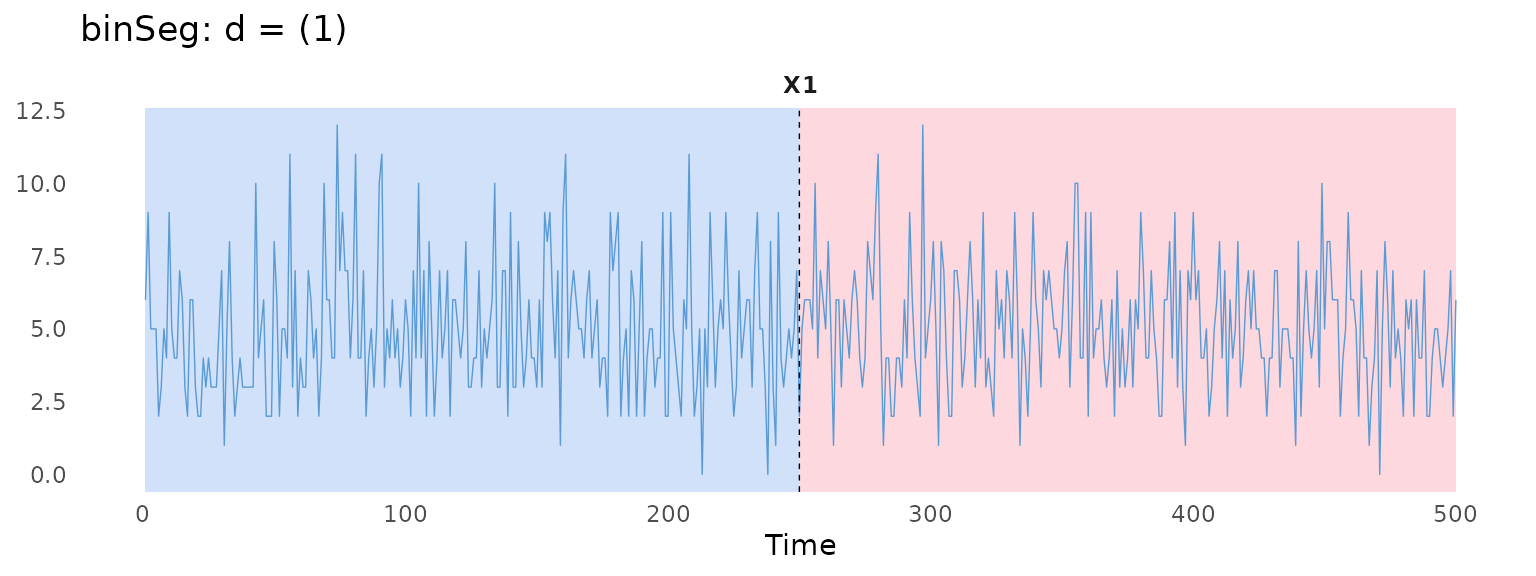
Here, counts contains a change-point at 250, but counts2 does not. Since poissonCost implicitly uses counts rather than counts2, the detected segmentation can be inconsistent with the data supplied to $fit().

binSegObj$plot()