Model selection

This chapter shows how to choose the number of change-points without tuning pen directly: by reading the cost trajectory (the elbow method), or by asking Dynp for the exact optimum for each count. To tune pen itself instead, for example with PELT, which has no elbow plot, see the case study Tuning the penalty.

library(rupturesRcpp)

Elbow method

binSeg and Window both build up their segmentation by adding one change-point at a time: binSeg by recursively splitting the segment that most reduces cost, Window by ranking candidate local maxima by gain. $getHistory() exposes that trajectory directly, so you can inspect it, or choose the number of change-points via the “elbow method”, instead of only tuning pen.

The examples below use the piecewise VAR series from Change in autoregressive dynamics:

set.seed(1)
tsMat = matrix(c(filter(rnorm(100), filter = 0.9, method = "recursive"),
                 filter(rnorm(100), filter = -0.9, method = "recursive")))

binSegObj = binSeg$new(minSize = 1L, jump = 1L, costFunc = costFunc$new("VAR"))
binSegObj$fit(tsMat)
#> Warning in private$.binSegModule$fit(): Some systems seem singular! Switch to
#> the approximate arma::solve()!
head(binSegObj$getHistory())
#>   k     cost added_bkp
#> 1 0 533.9504        NA
#> 2 1 165.2573        99
#> 3 2 159.6331       111
#> 4 3 154.7607       159
#> 5 4 149.1974       180
#> 6 5 144.7821       105

The warning is expected: with minSize = 1L, some candidate segments have too few observations to fit the VAR model, so their cost falls back to an approximate solve.

$plotElbow() renders this as a ggplot object (cost vs. number of change-points); look for where the marginal decrease in cost flattens out to pick k.

binSegObj$plotElbow(maxK = 10)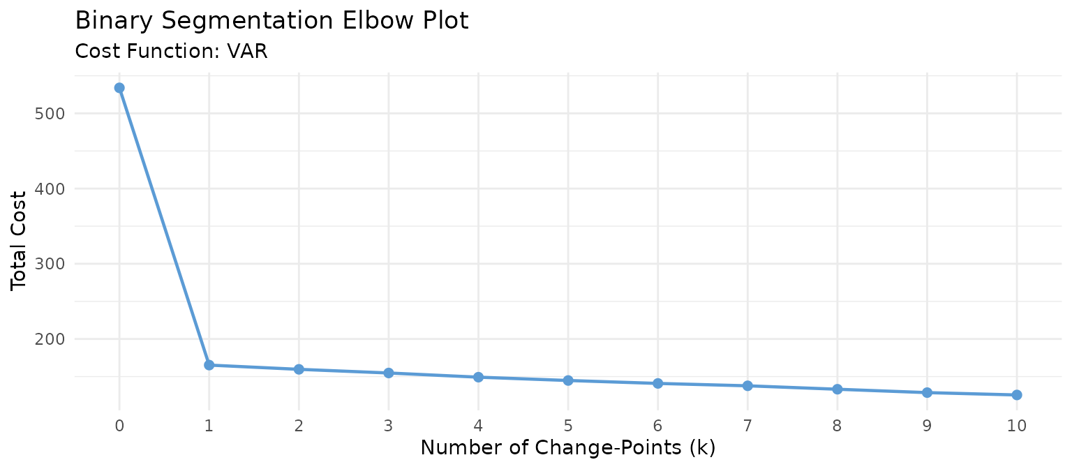

Once a k is chosen, $predict() accepts it directly via nBkps, which takes precedence over pen when both are supplied:

binSegObj$predict(nBkps = 1)
#> [1]  99 200

nBkps is treated as an upper bound, not a strict requirement: for binSeg it returns its own best answer among the splits it already explored, and for Window the nBkps highest-gain local maxima it found. Neither is guaranteed to be the globally optimal segmentation for that count. Window in particular can only ever offer as many change-points as it found local maxima for; if you ask for more, $predict() returns what’s available and reports the shortfall via a message rather than erroring.

Exact segmentation with Dynp

The caveat above (binSeg/Window returning their own best answer for a given nBkps, not necessarily the globally optimal one) is exactly what Dynp addresses. It finds the segmentation that is exactly optimal for a specified number of change-points, by building a full dynamic-programming table instead of searching greedily. The cost is complexity: the table takes O(nBkpsMax * M^2) time, where M is the number of (minSize, jump)-admissible positions, versus binSeg’s near-O(n log n) greedy search or PELT’s pruned search for a penalty.

set.seed(1121)
signals = as.matrix(c(rnorm(100, 0, 1), rnorm(100, 5, 1)))

DynpObj = Dynp$new(minSize = 1L, jump = 1L) # nBkpsMax left NULL -> resolved at $fit()
DynpObj$fit(signals)
#> `nBkpsMax` not set; using 20L.

$describe() shows the two fields specific to Dynp: the user-set nBkpsMax (here left NULL) and the resolvedNBkpsMax actually used, capped at 20 by default.

DynpObj$describe(printConfig = TRUE)
#> Exact Dynamic Programming (Dynp) 
#> minSize          : 1L
#> jump             : 1L
#> nBkpsMax         : NULL (auto)
#> resolvedNBkpsMax : 20L
#> costFunc         : "L2"
#> fitted           : TRUE
#> n                : 200L
#> p                : 1L

$predict(), $eval(), and $plot() all work exactly as with binSeg/Window/PELT, either via nBkps or via a penalty:

DynpObj$predict(nBkps = 1)
#> [1] 100 200

DynpObj$predict(pen = 100) # same split, reached via a penalty instead
#> [1] 100 200

DynpObj$plot(main = "method: Dynp; costFunc: L2; nBkps: 1")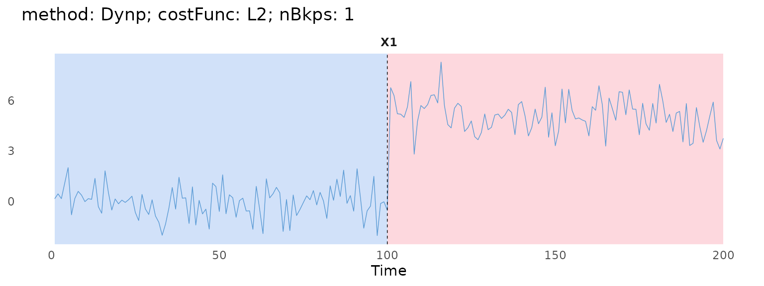

Since $fit() already computes the exact minimal cost for every change-point count from 0 to nBkpsMax in one pass (exposed via $costPath()), $getHistory()/$plotElbow() come for free here; no extra search is needed the way binSeg/Window would need to keep growing their own nested sequence:

head(DynpObj$getHistory())
#>   k      cost
#> 1 0 1511.6991
#> 2 1  186.6857
#> 3 2  176.1339
#> 4 3  169.4885
#> 5 4  163.1693
#> 6 5  158.4455

Unlike binSeg/Window, there is no added_bkp column: each k’s solution is independently exact and need not be nested inside the solution for k+1, so “the one breakpoint added at this step” is not generally well-defined. Use $predict(nBkps = k) to get the full breakpoint set for a given k.