Tuning the penalty

This case study chooses pen for PELT with the "L2" cost. It runs PELT over a grid of penalty values, records the number of change-points for each, and picks a pen where that number is stable.

This is useful when you would rather not use the methods in Model selection, or when the method has no elbow plot. PELT only returns the segmentation for a given pen, so it has no $getHistory() or $plotElbow().

library(rupturesRcpp)

We simulate a series with three changes in mean, at 100, 200 and 300.

set.seed(1)
tsMat = as.matrix(c(rnorm(100, 0), rnorm(100, 4), rnorm(100, 1), rnorm(100, 5)))

PELTObj = PELT$new(minSize = 1L, jump = 1L, costFunc = costFunc$new("L2"))
PELTObj$fit(tsMat)

Number of change-points against pen

The grid is evenly spaced on a log scale. It starts at 5, which is small enough to let noise in. It ends at the cost of the whole series with no change-point, given by $eval(). With a larger pen, any change-point costs more than it can save, so PELT returns none.

maxPen = PELTObj$eval(0, nrow(tsMat))
pens = exp(seq(log(5), log(maxPen), length.out = 50))
nCps = sapply(pens, function(pen) length(PELTObj$predict(pen = pen)) - 1)

$predict() returns the end-points, including n, so the number of change-points is one less than its length. The object is fitted once, so each pen only needs a new $predict().

plot(pens, nCps, type = "s", log = "x",
     xlab = "pen (log scale)", ylab = "Number of change-points")

A small pen lets noise through as extra change-points. A very large pen drops the true ones. In between, the number of change-points stays the same over a wide range of pen. That plateau is what we look for.

Picking pen from the plateau

We take the longest run of equal counts, and the pen in the middle of it.

runs = rle(nCps)
i = which.max(runs$lengths)
last = cumsum(runs$lengths)[i]
first = last - runs$lengths[i] + 1
penChosen = pens[(first + last) %/% 2]
c(nCps = runs$values[i], from = pens[first], to = pens[last], pen = penChosen)
#>       nCps       from         to        pen 
#>   3.000000   5.651823 364.433734  45.384082

The plateau is at 3 change-points, the true number. PELT is exact, so every pen on the plateau gives the same change-points.

PELTObj$predict(pen = penChosen)
#> [1] 100 200 300 400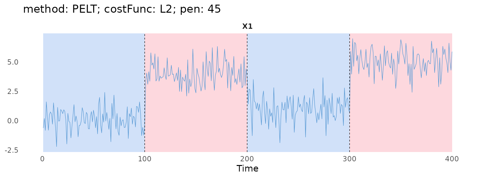

PELTObj$plot(main = paste0("method: PELT; costFunc: L2; pen: ", round(penChosen)))

The longest run is a simple rule. Look at the plot too: a short plateau, or two of similar length, means the data do not point to one clear number of change-points.