Change in autoregressive dynamics

This case study detects a change in autoregressive dynamics with the "VAR" cost and binSeg, and shows how to change an existing object through its active bindings. The series is piecewise vector autoregressive with constant noise variance.

library(rupturesRcpp)

set.seed(1)
tsMat = matrix(c(filter(rnorm(100), filter = 0.9, method = "recursive"),
                 filter(rnorm(100), filter = -0.9, method = "recursive")))

Suppose a binSeg object has already been fitted with the "L2" cost:

binSegObj = binSeg$new(minSize = 1L, jump = 1L, costFunc = costFunc$new("L2"))
binSegObj$fit(tsMat)

Here, the most suitable cost function is "VAR". We will modify the current binSegObj as follows:

VARObj = costFunc$new("VAR")
binSegObj$costFunc = VARObj
#> `costFunc` has been updated. Re-fitting the model.
#> Warning in private$.binSegModule$fit(): Some systems seem singular! Switch to
#> the approximate arma::solve()!

Modifying costFunc (or any other binding, such as tsMat) automatically triggers self$fit() once the object has been fitted.

binSegObj$describe(printConfig = TRUE)
#> Binary Segmentation (binSeg) 
#> minSize      : 1L
#> jump         : 1L
#> costFunc     : "VAR"
#> pVAR         : 1L
#> fitted       : TRUE
#> n            : 200L
#> p            : 1L

We can then perform binary segmentation with pen = 25, set by hand, and plot the segmentation results. See Tuning the penalty for how pen could be tuned.

binSegObj$predict(pen = 25)
#> [1]  99 200
binSegObj$plot(d = 1L,
               main = "method: binSeg; costFunc: VAR; pen: 25")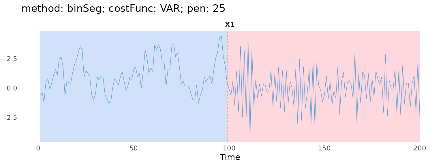

The warning is expected: with minSize = 1L, some candidate segments have too few observations to fit the VAR model, so their cost falls back to an approximate solve.

Instead of setting pen, we can choose the number of change-points with the elbow method (see Model selection). $plotElbow() plots the cost against the number of change-points.

binSegObj$plotElbow(maxK = 10)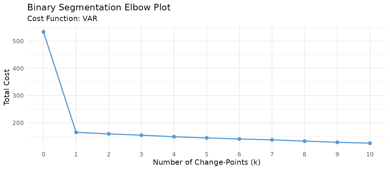

The cost drops sharply at one change-point and then levels off, so we take nBkps = 1. This gives the same change-point as pen = 25.

binSegObj$predict(nBkps = 1)
#> [1]  99 200